Page Contents
- Code Overview
- Easy Hydro Tests
- Harder Hydro Tests
- Tests with Viscosity
- Planet-Disk Tests

Disco solves hydrodynamic-like equations in conservation-law form:
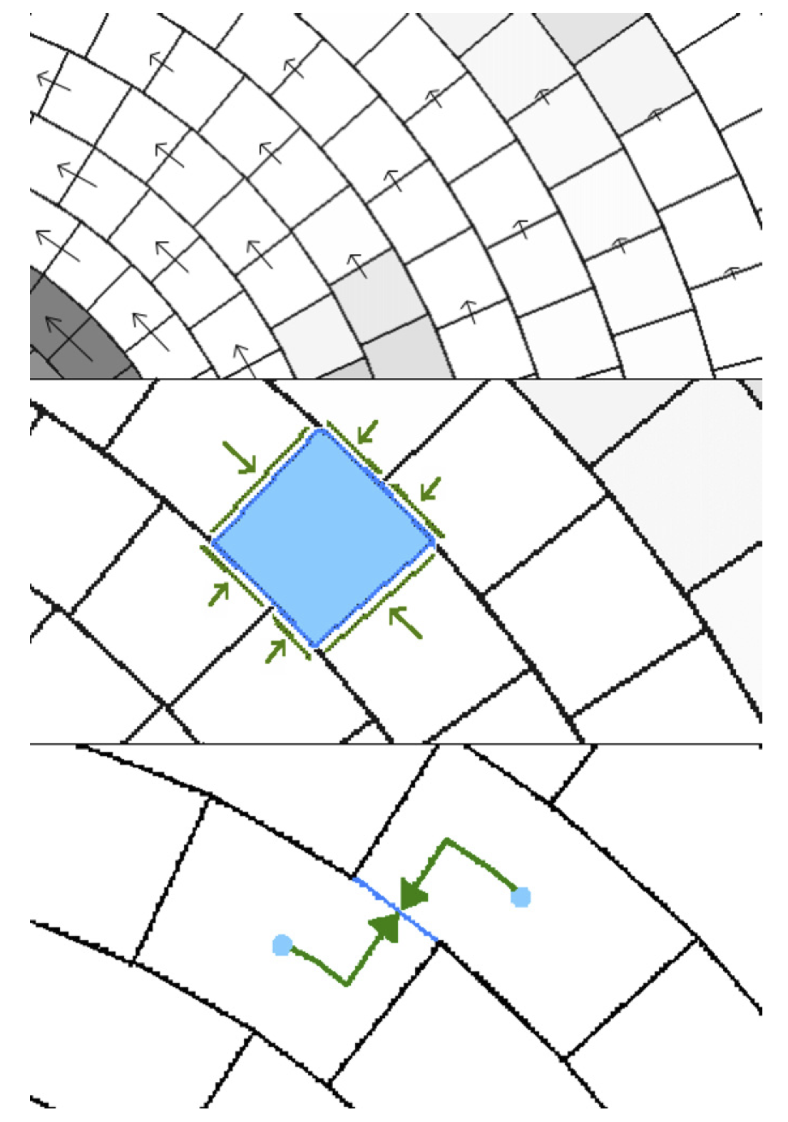
It does so using a moving cylindrical mesh. The conserved quantities (u) are averaged over wedge-like volumes, and the fluxes (F) are averaged over space and time on the interfaces between adjacent volumes. Averaging the above conservation law over a wedge and over time gives:
where the sum is over all faces attached to a given zone, and the index 'j' means the quantity is evaluated on face j. Now, if some of these faces are allowed to move with velocity
where
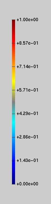
  if( val < .1 ){
     bbb = 4.*(val+.125);
     ggg = 0.0;
     rrr = 0.0;
  }else if( val < .375){
     bbb = 1.0;
     ggg = 4.*(val-.125);
     rrr = 0.0;
  }else if( val < .625 ){
     bbb = 4.*(.625-val);
     rrr = 4.*(val-.375);
     ggg = bbb;
     if( rrr > bbb ) ggg = rrr;
  }else if( val < .875){
     bbb = 0.0;
     ggg = 4.*(.875-val);
     rrr = 1.;
  }else{
     bbb = 0.0;
     ggg = 0.0;
     rrr = 4.*(1.125-val);
  }
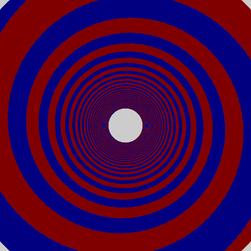
This test demonstrates Disco's ability to capture radially propagating shocks. For characteristics moving radially, Disco performs as a robust high-resolution shock-capturing code, even though the mesh motion is not employed.
It is also generally convenient to have a 2D shock solution to compare with numerically, which is why we have provided the numerical solution at high resolution.
Our domain extends from
We employ an adiabatic index of
Left State:
Right State:
We run this until a time
Numerical Solution (8192 radial zones)
On the right we plot the density at this time, for a resolution of 128 radial zones.
The isentropic pulse is a very simple nonlinear test for convergence of any code. We have set up a particular example and provided a high-resolution output which may be used as a basic code test. Convergence is easily checked by measuring entropy conservation. The initial setup is as follows:
For this problem, we choose an adiabatic index of
We therefore calculate the error simply by verifying entropy conservation at a time
We find fast convergence for this problem; for resolutions lower than 1024, we converge faster than second order. At higher resolutions, we converge at second order.
Numerical Solution (1024 radial zones)
This test is effectively 1D, as all motion is radial; it can be run with arbitrarily low angular resolution.
The test can also be used as a multidimensional test problem, simply by offsetting the origin of the pulse. We ran this problem with an origin offset by
Isentropic Pulse at t = 0.1. The top plot shows the density for a run with 64 radial zones compared with a high-resolution run. The bottom plot shows the second-order convergence of L1 error (defined in the test description).
A multidimensional version of the same test, which provides a simple nonaxisymmetric convergence test.
This test helps to demonstrate convergence, and the effectiveness of the Disco code at preservation of contact discontinuities.
The initial conditions are set so that centrifugal forces balance pressure gradients:
The vortex is trans-sonic (maximum Mach number of about 0.53). We calculate the error at
Plotting this data, we see clear second-order convergence. In the plots on the right, we include a passive scalar to demonstrate the code's ability to maintain contact discontinuities and prevent artificial diffusion. When mesh motion is turned off, the contact discontinuity is significantly smeared out. With mesh motion turned on, we maintain the contact discontinuity very precisely. A calculation at a resolution of 256 radial zones is also included for comparison.
Smooth vortex Test at t = 10. Red and Blue represent a passive scalar added to the initial conditions in order to visualize the Kepler flow. Top plot uses 22 radial zones with fixed mesh, center plot uses 22 radial zones with mesh motion turned on, and the final plot shows the high-resolution version (256 radial zones).
L1 error in density, computed at t = 10 (same time as the plots above). Data file in description.
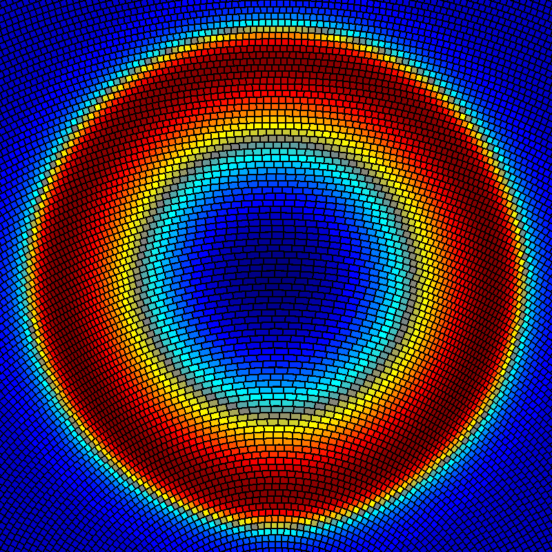
This is an extremely important test, as most of the real problems we wish to study have a Keplerian background flow. This stationary flow must be captured very accurately if we wish to study some subtle phenomenon which is added on top of this flow.
The setup for this problem is as follows:
Boundary conditions are simply fixed at these initial conditions. A point mass is of course inserted at r = 0 so that centrifugal and gravitational forces are balanced. The equation of state is adiabatic, with index
This gives a disk with a Mach number of 7.7 at the outer boundary, and 24.5 at the inner boundary.
Error is computed identically to the vortex problem. This is computed at a time
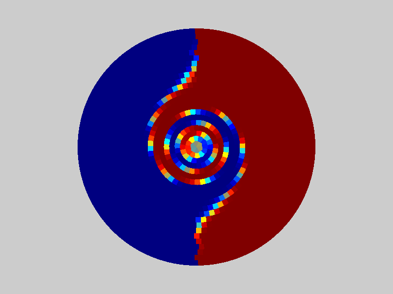
Because this test is axisymmetric (and therefore effectively 1D), it is not very important that the zones move with the flow. However, for demonstration purposes we have added a passive scalar to the initial conditions:
This passive scalar is plotted at time
Because this problem is highly supersonic, most of the energy is kinetic, meaning that small relative errors in the energy density can lead to large errors in the pressure. For this reason, it is extremely beneficial to evolve a modified energy density:
where
The tradeoff here is that energy is no longer conserved to machine precision, because the equations now have source terms involving
Keplerian Shear Flow Test with 512 Radial Zones, after one orbit at the outer radius (10^1.5 ~ 32 orbits at the inner radius). Red and Blue represent a passive scalar added to the initial conditions in order to visualize the Kepler flow.
L1 error in density, computed after half an orbit at the outer radius (~16 orbits at the inner radius). Data file in description.
Kelvin Helmholtz
if
if

Density at t = 2.0, after KH has begun to develop. Below, we compare fixed mesh vs. moving mesh. Contact discontinuities are much better preserved when the moving mesh is employed; advection errors wash out some of the features when the mesh is fixed. For this test, we use 128 uniformly distributed radial zones.
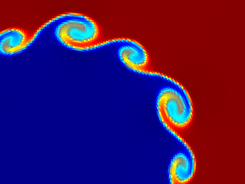
Fixed Mesh.
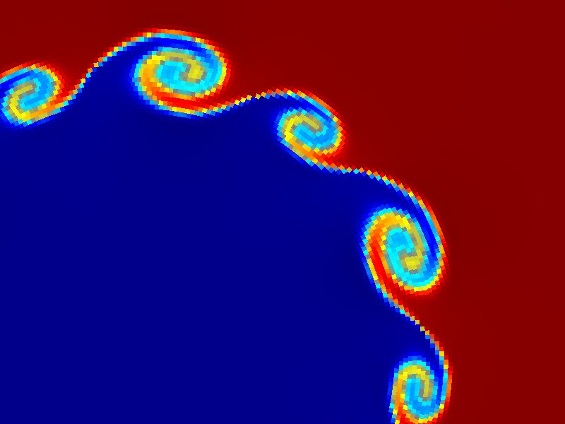
Moving Mesh.
In order to test Disco's implementation of viscosity, we need to perform a noncircular viscosity test. This is so that every term in the viscous equations is used. Fortunately, this is simple; all we need to do is set up a cartesian test problem and put it on our cylindrical grid. Of course, the cylindrical grid is certainly not ideal for this test, but the point of this test is to make sure all of our terms are implemented correctly, not to get extremely accurate results.
In cartesian coordinates, if we set up a flow with uniform density and pressure and with
where
We evolve this solution using the following parameters:
We start with the solution at time
We also played with the various viscous fluxes and source terms in cylindrical coordinates, and found that all of these terms are necessary to capture this solution to this accuracy. Therefore, this test is an excellent way of being sure the viscosity is implemented correctly.
Really ugly figure showing the cartesian shear flow test with 64 radial zones at t=1.0.
This gives a disk orbiting at about Mach 45 in the vicinity of
We wrote a simple 1D solver for this equation so that we can easily compare with Disco's performance on this problem. Of course, analytic Green's function solutions exist to this simple linear PDE, but I found it easier to solve the PDE numerically, that way I could easily choose whatever initial conditions I wanted and I didn't have to bother with any Bessel functions. For the initial conditions stated above for the surface density, we got the following solution at t = 100 by integrating this PDE:
This is plotted on the panel to the right, compared with Disco's solution using 64 radial zones. The solutions do not seem to match identically, but this could be due to thin-disk assumptions made in deriving the 1D equation, or due to viscous heating, as we did not explicitly enforce isothermality. It could also possibly be due to the explicit form of the viscous terms in the hydro equations. At any rate, errors appear to be at the percent-level.
Viscous disk at t=100 using 64 radial zones. It's not perfect, which annoys me.
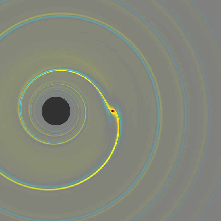
It is important to be able to capture planet-disk interactions in a highly idealized context. We look at the linear interaction between an Earth-mass planet and a supersonic Keplerian disk whose Mach number is
Here, to simplify the problem, we use a nearly isothermal equation of state:
with boundary conditions fixed at the initial conditions. So far, this is just a supersonic Keplerian disk, similar to the test done above (except with a softer equation of state). The only additional ingredient is a point mass orbiting at
We use the Earth-to-Sun mass ratio:
where I have defined
The potential is of a point gravitating mass with smoothing length
where
The simplest analytic comparison is given by the spiral wave produced by the planet. It is straightforward to calculate the shape of this wave from linear theory:
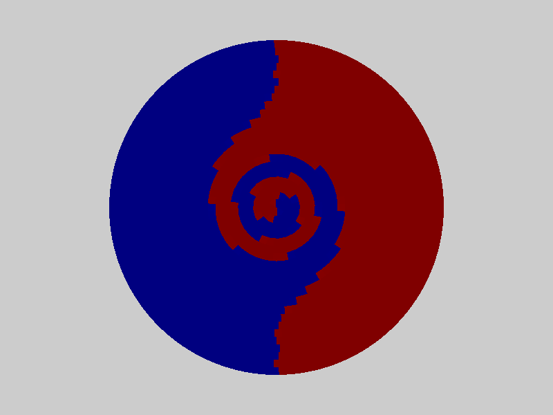
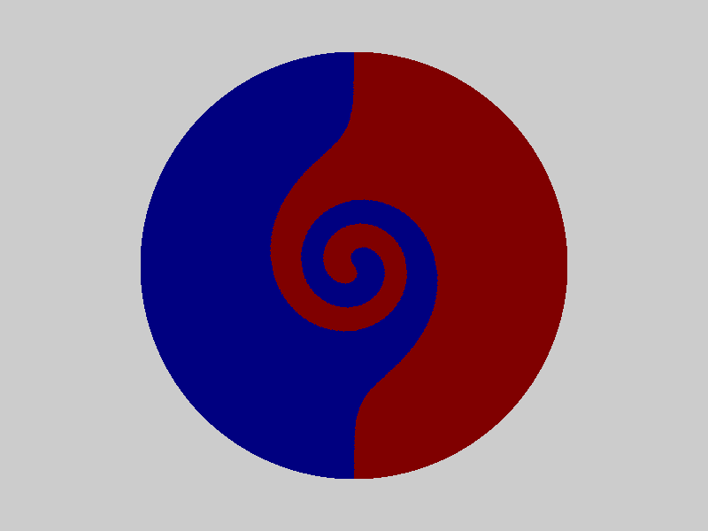
The spiral wave is quickly established in the first orbit. See figure.

256 radial zones after a single orbit. Density fluctuations range from -1% to +4%